Belarusian - Wikilangs Models

Comprehensive Research Report & Full Ablation Study

This repository contains NLP models trained and evaluated by Wikilangs, specifically on Belarusian Wikipedia data. We analyze tokenizers, n-gram models, Markov chains, vocabulary statistics, and word embeddings.

📋 Repository Contents

Models & Assets

• Tokenizers (8k, 16k, 32k, 64k)
• N-gram models (2, 3, 4, 5-gram)
• Markov chains (context of 1, 2, 3, 4 and 5)
• Subword N-gram and Markov chains
• Embeddings in various sizes and dimensions (aligned and unaligned)
• Language Vocabulary
• Language Statistics

Analysis and Evaluation

• 1. Tokenizer Evaluation
• 2. N-gram Model Evaluation
• 3. Markov Chain Evaluation
• 4. Vocabulary Analysis
• 5. Word Embeddings Evaluation
• 6. Morphological Analysis (Experimental)
• 7. Summary & Recommendations
• Metrics Glossary
• Visualizations Index

---

1. Tokenizer Evaluation

Results

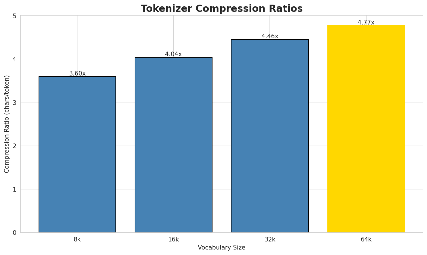
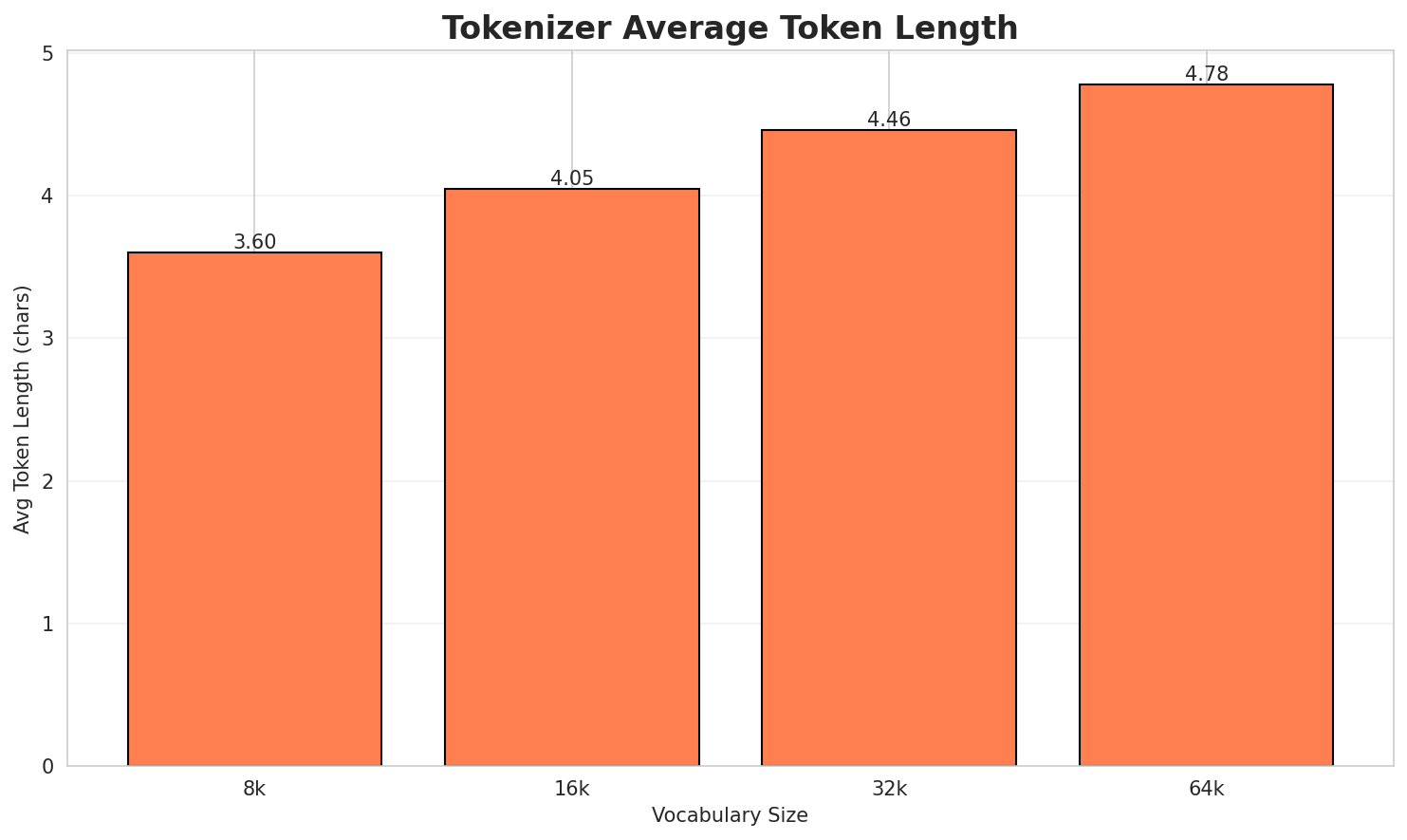
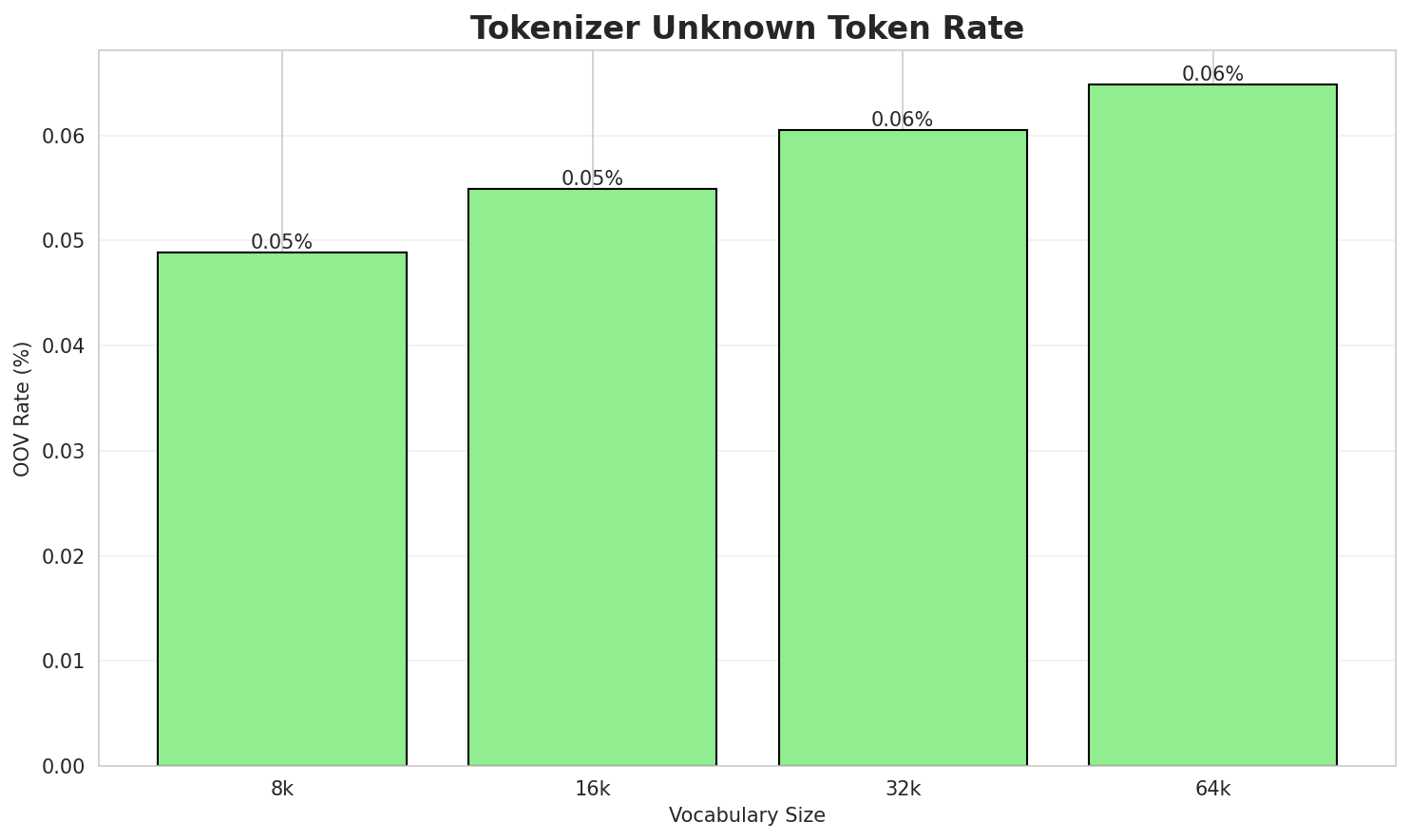
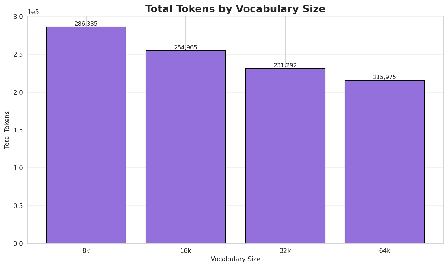
Vocab Size	Compression	Avg Token Len	UNK Rate	Total Tokens
8k	3.599x	3.60	0.0489%	286,335
16k	4.042x	4.05	0.0549%	254,965
32k	4.455x	4.46	0.0605%	231,292
64k	4.771x 🏆	4.78	0.0648%	215,975

Tokenization Examples

Below are sample sentences tokenized with each vocabulary size:

Sample 1: Ланавычы () — вёска ў Самбірскім раёне Львоўскай вобласці Украіны. Крыніцы пункт...

Vocab	Tokens	Count
8k	▁ла на вы чы ▁() ▁— ▁вёска ▁ў ▁сам бі ... (+12 more)	22
16k	▁ла на вы чы ▁() ▁— ▁вёска ▁ў ▁сам бі ... (+12 more)	22
32k	▁ла на вычы ▁() ▁— ▁вёска ▁ў ▁самбі рскім ▁раёне ... (+9 more)	19
64k	▁лана вычы ▁() ▁— ▁вёска ▁ў ▁самбірскім ▁раёне ▁львоўскай ▁вобласці ... (+6 more)	16

Sample 2: Марсо () — французскае прозвішча. Вядомыя носьбіты Марсель Марсо, французскі арт...

Vocab	Tokens	Count
8k	▁мар со ▁() ▁— ▁француз скае ▁прозвішча . ▁вядомыя ▁носьбіты ... (+17 more)	27
16k	▁мар со ▁() ▁— ▁француз скае ▁прозвішча . ▁вядомыя ▁носьбіты ... (+16 more)	26
32k	▁мар со ▁() ▁— ▁француз скае ▁прозвішча . ▁вядомыя ▁носьбіты ... (+15 more)	25
64k	▁мар со ▁() ▁— ▁французскае ▁прозвішча . ▁вядомыя ▁носьбіты ▁марсель ... (+14 more)	24

Sample 3: Вораніў () — вёска ў Гарадэнкіўскім раёне Івана-Франкоўскай вобласці Украіны. Кр...

Vocab	Tokens	Count
8k	▁вора ніў ▁() ▁— ▁вёска ▁ў ▁гарад эн кі ўскім ... (+21 more)	31
16k	▁вора ніў ▁() ▁— ▁вёска ▁ў ▁гарад эн кіўскім ▁раёне ... (+18 more)	28
32k	▁вора ніў ▁() ▁— ▁вёска ▁ў ▁гарад эн кіўскім ▁раёне ... (+17 more)	27
64k	▁вора ніў ▁() ▁— ▁вёска ▁ў ▁гарад эн кіўскім ▁раёне ... (+17 more)	27

Key Findings

• Best Compression: 64k achieves 4.771x compression
• Lowest UNK Rate: 8k with 0.0489% unknown tokens
• Trade-off: Larger vocabularies improve compression but increase model size
• Recommendation: 32k vocabulary provides optimal balance for production use

---

2. N-gram Model Evaluation

Results

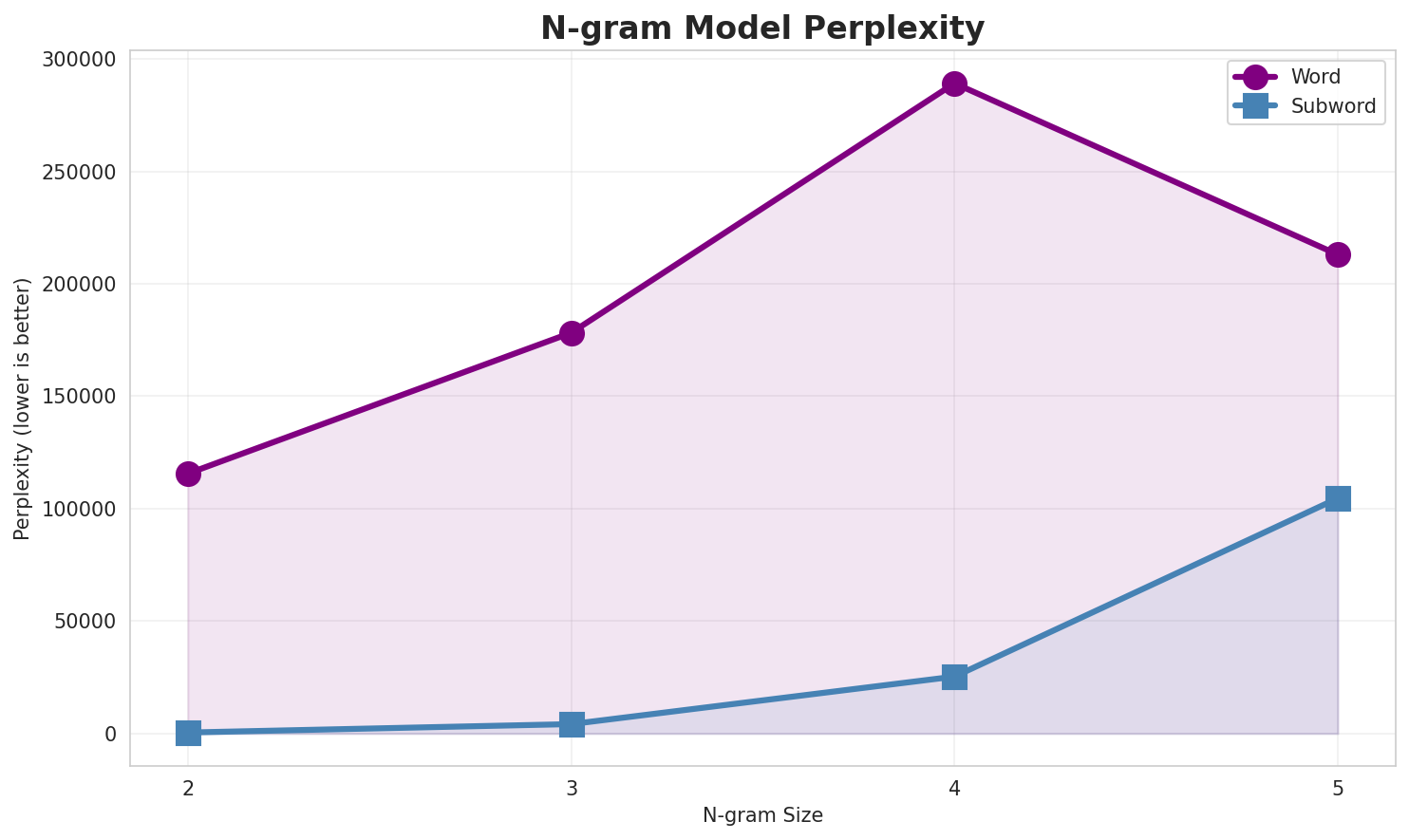
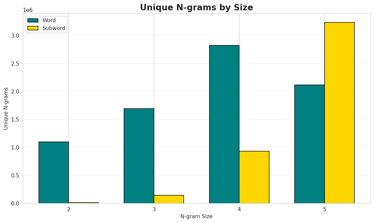
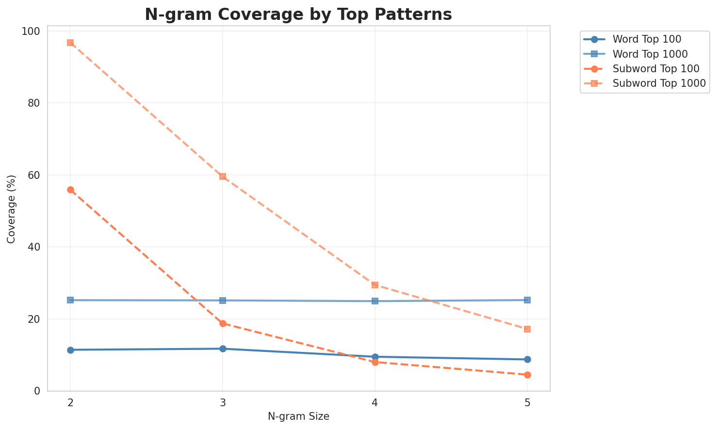
N-gram	Variant	Perplexity	Entropy	Unique N-grams	Top-100 Coverage	Top-1000 Coverage
2-gram	Word	115,602	16.82	1,101,685	11.4%	25.2%
2-gram	Subword	453 🏆	8.82	15,623	55.9%	96.8%
3-gram	Word	178,210	17.44	1,692,602	11.7%	25.1%
3-gram	Subword	4,191	12.03	146,010	18.7%	59.5%
4-gram	Word	289,150	18.14	2,823,610	9.4%	24.9%
4-gram	Subword	25,327	14.63	932,448	8.0%	29.4%
5-gram	Word	212,986	17.70	2,118,708	8.7%	25.2%
5-gram	Subword	104,621	16.67	3,234,164	4.5%	17.2%

Top 5 N-grams by Size

2-grams (Word):

Rank	N-gram	Count
1	0 10	188,589
2	10 0	184,434
3	0 09	178,217
4	09 0	172,685
5	у годзе	141,829

3-grams (Word):

Rank	N-gram	Count
1	0 10 0	183,055
2	0 09 0	171,685
3	0 11 0	133,047
4	0 08 0	125,665
5	0 07 0	84,761

4-grams (Word):

Rank	N-gram	Count
1	0 44 0 10	28,229
2	44 0 10 0	27,892
3	0 47 0 10	27,125
4	47 0 10 0	26,709
5	0 50 0 10	26,628

5-grams (Word):

Rank	N-gram	Count
1	0 44 0 10 0	27,892
2	0 47 0 10 0	26,707
3	0 50 0 10 0	26,249
4	0 45 0 10 0	25,524
5	0 49 0 10 0	24,716

2-grams (Subword):

Rank	N-gram	Count
1	а _	7,411,164
2	н а	5,858,867
3	р а	5,764,007
4	к а	4,983,576
5	_ п	4,779,657

3-grams (Subword):

Rank	N-gram	Count
1	_ п а	2,113,963
2	_ 0 ,	1,872,411
3	_ н а	1,678,358
4	н а _	1,430,853
5	_ п р	1,351,115

4-grams (Subword):

Rank	N-gram	Count
1	а г а _	985,197
2	_ п р а	752,091
3	_ г о д	714,067
4	_ н а _	694,537
5	к а й _	548,513

5-grams (Subword):

Rank	N-gram	Count
1	к а г а _	467,479
2	с к а й _	409,977
3	с к а г а	393,058
4	б е л а р	392,561
5	е л а р у	392,043

Key Findings

• Best Perplexity: 2-gram (subword) with 453
• Entropy Trend: Decreases with larger n-grams (more predictable)
• Coverage: Top-1000 patterns cover ~17% of corpus
• Recommendation: 4-gram or 5-gram for best predictive performance

---

3. Markov Chain Evaluation

Results

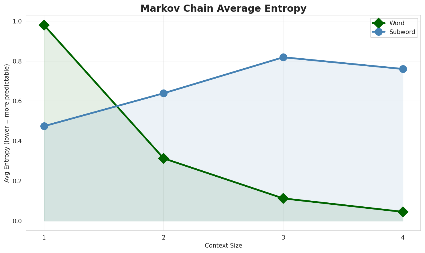
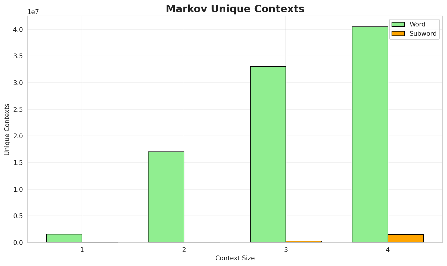
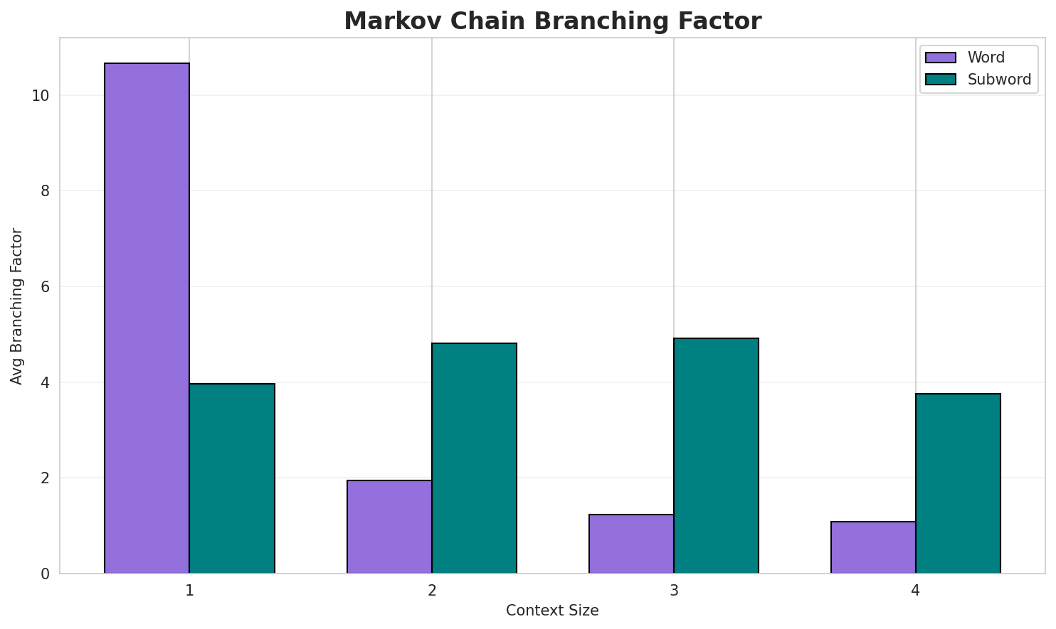
Context	Variant	Avg Entropy	Perplexity	Branching Factor	Unique Contexts	Predictability
1	Word	0.9802	1.973	10.66	1,600,794	2.0%
1	Subword	0.4743	1.389	3.96	16,475	52.6%
2	Word	0.3132	1.242	1.95	17,028,048	68.7%
2	Subword	0.6391	1.557	4.81	65,298	36.1%
3	Word	0.1128	1.081	1.23	33,045,925	88.7%
3	Subword	0.8191	1.764	4.91	313,830	18.1%
4	Word	0.0455 🏆	1.032	1.08	40,473,004	95.4%
4	Subword	0.7606	1.694	3.75	1,541,159	23.9%

Generated Text Samples (Word-based)

Below are text samples generated from each word-based Markov chain model:

Context Size 1:

1. 0 06 0 1 мінскай вобласці беларусі ў раёне віцебскай губерні земскага самакіравання якая выказалася ...
2. і дзіцячы сад каралевы якія выменьвалі ў эджбастане бірмінгем сіці манчэстэр юнайтэд дзе адносна нев...
3. у годзе стала ўскосным выглядзе шоу consecința istorică sibiu mitropolitul andrei yahorau alena маё ...

Context Size 2:

1. 0 10 0 34 0 12 0 38 0 11 0 53 0 09 0 41 0
2. 10 0 55 0 09 0 46 0 10 0 63 0 08 0 75 0 07
3. 0 09 0 54 0 09 0 47 0 10 0 48 0 10 0 45 0

Context Size 3:

1. 0 10 0 37 0 12 0 45 0 10 0 60 0 08 0 58 0 09
2. 0 09 0 54 0 09 0 50 0 09 so a 0 67 0 08 0 79
3. 0 11 0 47 0 10 0 54 0 09 0 48 0 10 0 43 0 11

Context Size 4:

1. 0 44 0 10 0 40 0 11 0 54 0 32 0 45 0 32 0 56 0
2. 44 0 10 0 47 0 10 0 48 0 10 0 48 0 10 0 57 0 06
3. 0 47 0 10 0 54 0 09 0 87 0 06 sbbc 0 78 0 07 0 47

Generated Text Samples (Subword-based)

Below are text samples generated from each subword-based Markov chain model:

Context Size 1:

1. _бек»_мано_szk._
2. аёрларныкльбеніц
3. нагркаў_вай_stol

Context Size 2:

1. а_вылкі_ў_парышша
2. на_апілік_вы,_які
3. раў_звагарскаў_вы

Context Size 3:

1. _памка:_ю._тайскаг
2. _0,53_0,42_0,43_0,
3. _насцю_і_тавіч_см.

Context Size 4:

1. ага_заняў_і_паведа,
2. _прасійскаў_супольс
3. _годзе_прыезда_філь

Key Findings

• Best Predictability: Context-4 (word) with 95.4% predictability
• Branching Factor: Decreases with context size (more deterministic)
• Memory Trade-off: Larger contexts require more storage (1,541,159 contexts)
• Recommendation: Context-3 or Context-4 for text generation

---

4. Vocabulary Analysis

Statistics

Metric	Value
Vocabulary Size	741,819
Total Tokens	55,243,342
Mean Frequency	74.47
Median Frequency	4
Frequency Std Dev	3873.91

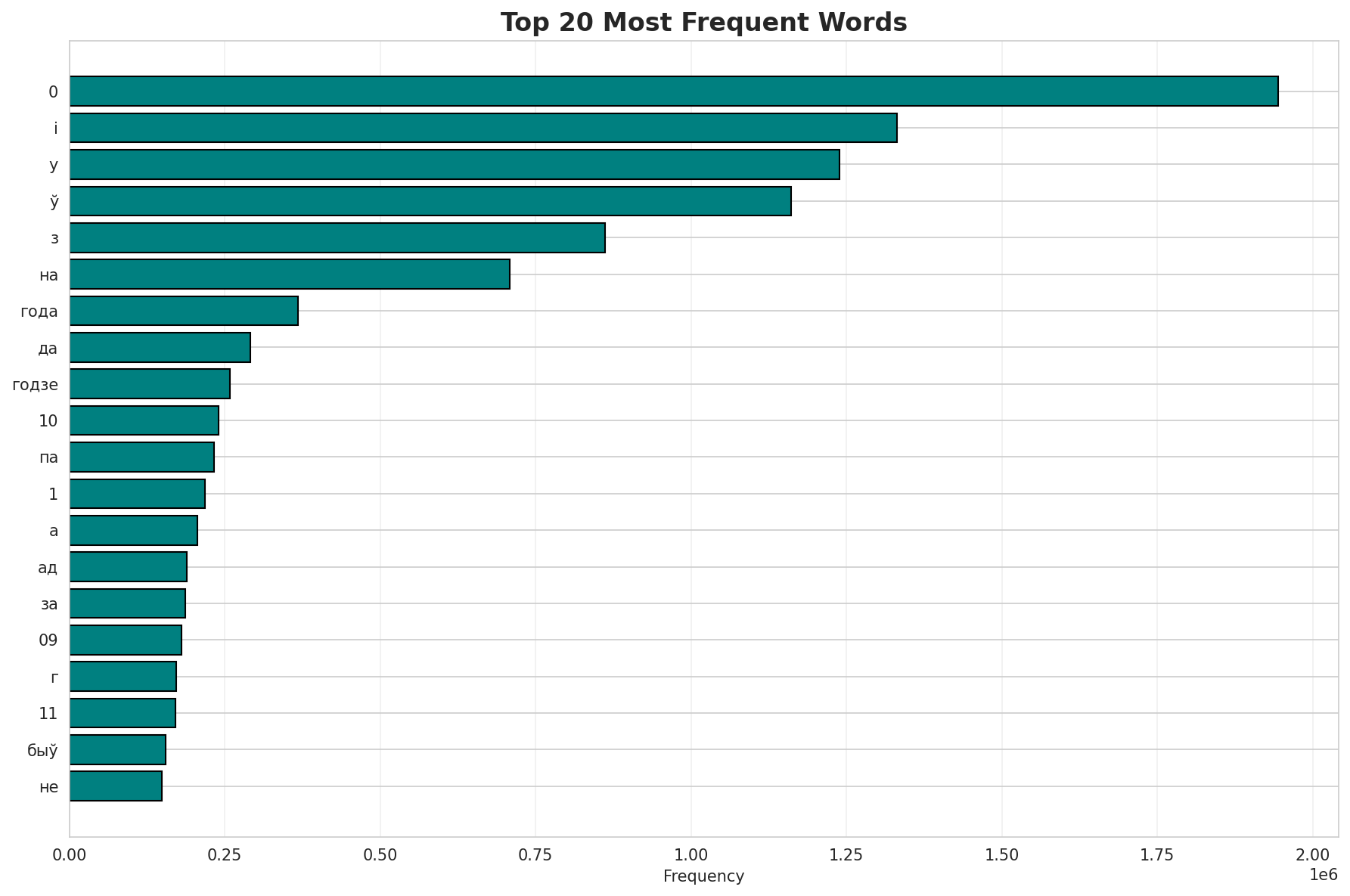
Most Common Words

Rank	Word	Frequency
1	0	1,944,910
2	і	1,331,350
3	у	1,238,468
4	ў	1,161,043
5	з	862,221
6	на	708,262
7	года	367,568
8	да	290,434
9	годзе	258,378
10	10	239,964

Least Common Words (from vocabulary)

Rank	Word	Frequency
1	девятке	2
2	дэкунаў	2
3	iovine	2
4	іавін	2
5	аёвіну	2
6	джэніка	2
7	мэрылінам	2
8	сардэшная	2
9	івасю	2
10	стеценко	2

Zipf's Law Analysis

Metric	Value
Zipf Coefficient	0.9714
R² (Goodness of Fit)	0.997383
Adherence Quality	excellent

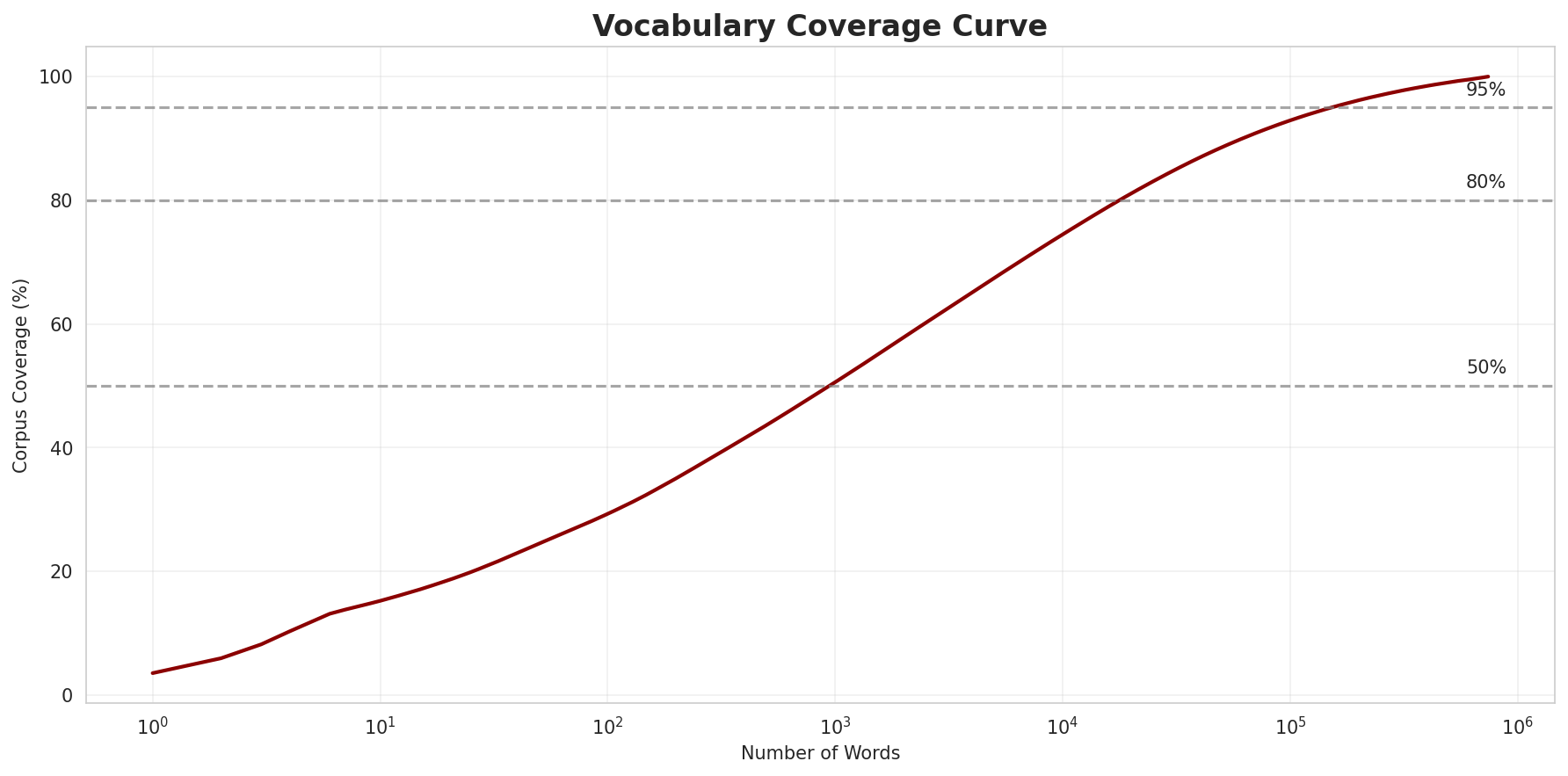
Coverage Analysis

Top N Words	Coverage
Top 100	29.3%
Top 1,000	50.6%
Top 5,000	67.4%
Top 10,000	74.5%

Key Findings

• Zipf Compliance: R²=0.9974 indicates excellent adherence to Zipf's law
• High Frequency Dominance: Top 100 words cover 29.3% of corpus
• Long Tail: 731,819 words needed for remaining 25.5% coverage

---

5. Word Embeddings Evaluation

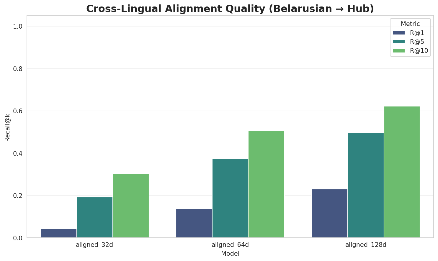
5.1 Cross-Lingual Alignment

5.2 Model Comparison

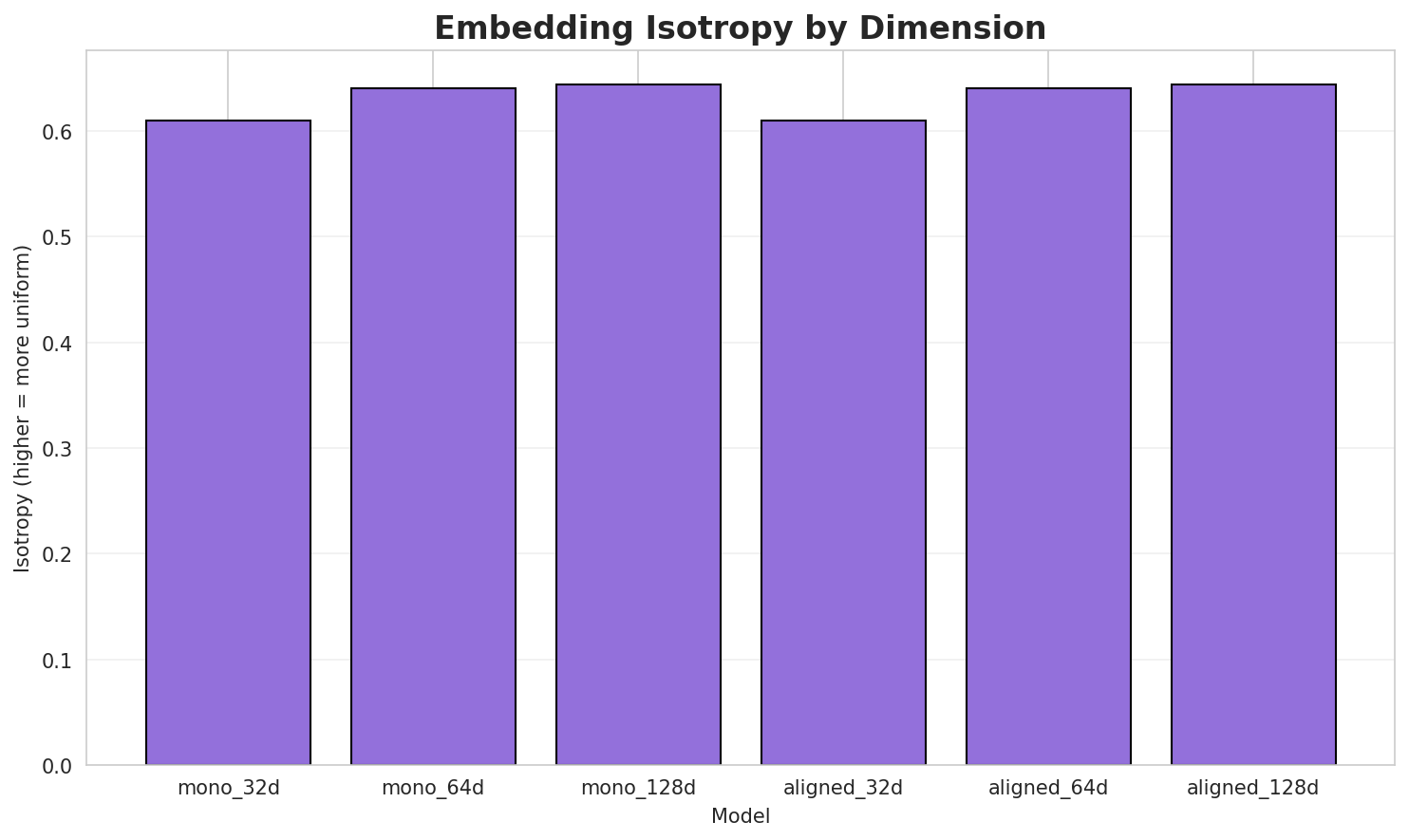
Model	Dimension	Isotropy	Semantic Density	Alignment R@1	Alignment R@10
mono_32d	32	0.6096	0.3533	N/A	N/A
mono_64d	64	0.6408	0.2859	N/A	N/A
mono_128d	128	0.6444	0.2271	N/A	N/A
aligned_32d	32	0.6096	0.3568	0.0440	0.3040
aligned_64d	64	0.6408	0.2908	0.1380	0.5080
aligned_128d	128	0.6444 🏆	0.2362	0.2300	0.6220

Key Findings

• Best Isotropy: aligned_128d with 0.6444 (more uniform distribution)
• Semantic Density: Average pairwise similarity of 0.2917. Lower values indicate better semantic separation.
• Alignment Quality: Aligned models achieve up to 23.0% R@1 in cross-lingual retrieval.
• Recommendation: 128d aligned for best cross-lingual performance

---

6. Morphological Analysis (Experimental)

This section presents an automated morphological analysis derived from the statistical divergence between word-level and subword-level models. By analyzing where subword predictability spikes and where word-level coverage fails, we can infer linguistic structures without supervised data.

6.1 Productivity & Complexity

Metric	Value	Interpretation	Recommendation
Productivity Index	5.000	High morphological productivity	Reliable analysis
Idiomaticity Gap	0.467	High formulaic/idiomatic content	-

6.2 Affix Inventory (Productive Units)

These are the most productive prefixes and suffixes identified by sampling the vocabulary for global substitutability patterns. A unit is considered an affix if stripping it leaves a valid stem that appears in other contexts.

Productive Prefixes

Prefix	Examples
-па	параллельной, падаплёка, падкіданні
-ка	канавалава, кафедрамі, калеснікава
-пр	прышчэпаўшчына, прыпяцкі, прапіткі

Productive Suffixes

Suffix	Examples
-а	гароха, прышчэпаўшчына, падаплёка
-га	паўднёвага, іпацеўскага, міжазёрнага
-кі	леанінскі, прыпяцкі, прапіткі
-ай	кіянкай, ольстэрскай, найноўшай
-ага	паўднёвага, іпацеўскага, міжазёрнага
-ая	рудэральная, прымененая, свальбардская
-аў	шакіраваў, вігаў, шукальнікаў
-на	прышчэпаўшчына, непэсрэдна, скампанавана

6.3 Bound Stems (Lexical Roots)

Bound stems are high-frequency subword units that are semantically cohesive but rarely appear as standalone words. These often correspond to the 'core' of a word that requires inflection or derivation to be valid.

Stem	Cohesion	Substitutability	Examples
анск	1.51x	1027 contexts	ганск, данск, канск
нска	1.55x	503 contexts	унска, янска, інская
насц	1.79x	190 contexts	насце, насця, насцю
асел	2.08x	87 contexts	асель, аселі, расел
елар	2.39x	47 contexts	белар, селар, гелар
ўска	1.58x	236 contexts	еўска, іўска, ёўскае
аецц	2.20x	48 contexts	маецца, каецца, лаецца
тычн	1.49x	233 contexts	этычны, стычня, этычна
нскі	1.34x	416 contexts	енскі, янскі, інскі
ельн	1.32x	342 contexts	ельню, ельна, ельні
ходз	1.47x	182 contexts	ходзі, ходза, ходзь
ання	1.47x	174 contexts	рання, вання, арання

6.4 Affix Compatibility (Co-occurrence)

This table shows which prefixes and suffixes most frequently co-occur on the same stems, revealing the 'stacking' rules of the language's morphology.

Prefix	Suffix	Frequency	Examples
-па	-а	57 words	падлічваюцца, павета
-ка	-а	51 words	карахана, каралькова
-пр	-а	33 words	прынцэса, працягваюцца
-па	-ыя	14 words	падпружныя, пасярэбраныя
-па	-ай	14 words	паўлавіцкай, пагібельнай
-ка	-ая	14 words	карнуая, карэспандэнцкая
-ка	-на	13 words	карахана, кадрына
-ка	-га	13 words	калевальскага, каларадскага
-па	-кі	13 words	пакупкі, палачанкі
-па	-га	13 words	папаленага, палаткавага

6.5 Recursive Morpheme Segmentation

Using Recursive Hierarchical Substitutability, we decompose complex words into their constituent morphemes. This approach handles nested affixes (e.g., prefix-prefix-root-suffix).

Word	Suggested Split	Confidence	Stem
галіцынаўка	галіцын-аў-ка	6.0	галіцын
перакладчыкаў	перакладчык-аў	4.5	перакладчык
зікуратаў	зікурат-аў	4.5	зікурат
астраблемай	астраблем-ай	4.5	астраблем
авіяатрадаў	авіяатрад-аў	4.5	авіяатрад
гукарадаў	гукарад-аў	4.5	гукарад
цырульнікаў	цырульнік-аў	4.5	цырульнік
адпраўшчыкаў	адпраўшчык-аў	4.5	адпраўшчык
рэдэмптарыстаў	рэдэмптарыст-аў	4.5	рэдэмптарыст
кулінараў	кулінар-аў	4.5	кулінар
іньігесаў	іньігес-аў	4.5	іньігес
гэлтахтаў	гэлтахт-аў	4.5	гэлтахт
рэгістрацыйна	рэгістрацый-на	4.5	рэгістрацый
чапаеўскага	чапаеўск-ага	4.5	чапаеўск
грунтоўка	грунтоў-ка	4.5	грунтоў

6.6 Linguistic Interpretation

Automated Insight: The language Belarusian shows high morphological productivity. The subword models are significantly more efficient than word models, suggesting a rich system of affixation or compounding.

Note on Idiomaticity: The high Idiomaticity Gap suggests a large number of frequent multi-word expressions or formulaic sequences that are statistically distinct from their component parts.

---

7. Summary & Recommendations

Production Recommendations

Component	Recommended	Rationale
Tokenizer	64k BPE	Best compression (4.77x)
N-gram	2-gram	Lowest perplexity (453)
Markov	Context-4	Highest predictability (95.4%)
Embeddings	100d	Balanced semantic capture and isotropy

---

Appendix: Metrics Glossary & Interpretation Guide

This section provides definitions, intuitions, and guidance for interpreting the metrics used throughout this report.

Tokenizer Metrics

Compression Ratio

Definition: The ratio of characters to tokens (chars/token). Measures how efficiently the tokenizer represents text.

Intuition: Higher compression means fewer tokens needed to represent the same text, reducing sequence lengths for downstream models. A 3x compression means ~3 characters per token on average.

What to seek: Higher is generally better for efficiency, but extremely high compression may indicate overly aggressive merging that loses morphological information.

Average Token Length (Fertility)

Definition: Mean number of characters per token produced by the tokenizer.

Intuition: Reflects the granularity of tokenization. Longer tokens capture more context but may struggle with rare words; shorter tokens are more flexible but increase sequence length.

What to seek: Balance between 2-5 characters for most languages. Arabic/morphologically-rich languages may benefit from slightly longer tokens.

Unknown Token Rate (OOV Rate)

Definition: Percentage of tokens that map to the unknown/UNK token, indicating words the tokenizer cannot represent.

Intuition: Lower OOV means better vocabulary coverage. High OOV indicates the tokenizer encounters many unseen character sequences.

What to seek: Below 1% is excellent; below 5% is acceptable. BPE tokenizers typically achieve very low OOV due to subword fallback.

N-gram Model Metrics

Perplexity

Definition: Measures how "surprised" the model is by test data. Mathematically: 2^(cross-entropy). Lower values indicate better prediction.

Intuition: If perplexity is 100, the model is as uncertain as if choosing uniformly among 100 options at each step. A perplexity of 10 means effectively choosing among 10 equally likely options.

What to seek: Lower is better. Perplexity decreases with larger n-grams (more context). Values vary widely by language and corpus size.

Entropy

Definition: Average information content (in bits) needed to encode the next token given the context. Related to perplexity: perplexity = 2^entropy.

Intuition: High entropy means high uncertainty/randomness; low entropy means predictable patterns. Natural language typically has entropy between 1-4 bits per character.

What to seek: Lower entropy indicates more predictable text patterns. Entropy should decrease as n-gram size increases.

Coverage (Top-K)

Definition: Percentage of corpus occurrences explained by the top K most frequent n-grams.

Intuition: High coverage with few patterns indicates repetitive/formulaic text; low coverage suggests diverse vocabulary usage.

What to seek: Depends on use case. For language modeling, moderate coverage (40-60% with top-1000) is typical for natural text.

Markov Chain Metrics

Average Entropy

Definition: Mean entropy across all contexts, measuring average uncertainty in next-word prediction.

Intuition: Lower entropy means the model is more confident about what comes next. Context-1 has high entropy (many possible next words); Context-4 has low entropy (few likely continuations).

What to seek: Decreasing entropy with larger context sizes. Very low entropy (<0.1) indicates highly deterministic transitions.

Branching Factor

Definition: Average number of unique next tokens observed for each context.

Intuition: High branching = many possible continuations (flexible but uncertain); low branching = few options (predictable but potentially repetitive).

What to seek: Branching factor should decrease with context size. Values near 1.0 indicate nearly deterministic chains.

Predictability

Definition: Derived metric: (1 - normalized_entropy) × 100%. Indicates how deterministic the model's predictions are.

Intuition: 100% predictability means the next word is always certain; 0% means completely random. Real text falls between these extremes.

What to seek: Higher predictability for text generation quality, but too high (>98%) may produce repetitive output.

Vocabulary & Zipf's Law Metrics

Zipf's Coefficient

Definition: The slope of the log-log plot of word frequency vs. rank. Zipf's law predicts this should be approximately -1.

Intuition: A coefficient near -1 indicates the corpus follows natural language patterns where a few words are very common and most words are rare.

What to seek: Values between -0.8 and -1.2 indicate healthy natural language distribution. Deviations may suggest domain-specific or artificial text.

R² (Coefficient of Determination)

Definition: Measures how well the linear fit explains the frequency-rank relationship. Ranges from 0 to 1.

Intuition: R² near 1.0 means the data closely follows Zipf's law; lower values indicate deviation from expected word frequency patterns.

What to seek: R² > 0.95 is excellent; > 0.99 indicates near-perfect Zipf adherence typical of large natural corpora.

Vocabulary Coverage

Definition: Cumulative percentage of corpus tokens accounted for by the top N words.

Intuition: Shows how concentrated word usage is. If top-100 words cover 50% of text, the corpus relies heavily on common words.

What to seek: Top-100 covering 30-50% is typical. Higher coverage indicates more repetitive text; lower suggests richer vocabulary.

Word Embedding Metrics

Isotropy

Definition: Measures how uniformly distributed vectors are in the embedding space. Computed as the ratio of minimum to maximum singular values.

Intuition: High isotropy (near 1.0) means vectors spread evenly in all directions; low isotropy means vectors cluster in certain directions, reducing expressiveness.

What to seek: Higher isotropy generally indicates better-quality embeddings. Values > 0.1 are reasonable; > 0.3 is good. Lower-dimensional embeddings tend to have higher isotropy.

Average Norm

Definition: Mean magnitude (L2 norm) of word vectors in the embedding space.

Intuition: Indicates the typical "length" of vectors. Consistent norms suggest stable training; high variance may indicate some words are undertrained.

What to seek: Relatively consistent norms across models. The absolute value matters less than consistency (low std deviation).

Cosine Similarity

Definition: Measures angular similarity between vectors, ranging from -1 (opposite) to 1 (identical direction).

Intuition: Words with similar meanings should have high cosine similarity. This is the standard metric for semantic relatedness in embeddings.

What to seek: Semantically related words should score > 0.5; unrelated words should be near 0. Synonyms often score > 0.7.

t-SNE Visualization

Definition: t-Distributed Stochastic Neighbor Embedding - a dimensionality reduction technique that preserves local structure for visualization.

Intuition: Clusters in t-SNE plots indicate groups of semantically related words. Spread indicates vocabulary diversity; tight clusters suggest semantic coherence.

What to seek: Meaningful clusters (e.g., numbers together, verbs together). Avoid over-interpreting distances - t-SNE preserves local, not global, structure.

General Interpretation Guidelines

1. Compare within model families: Metrics are most meaningful when comparing models of the same type (e.g., 8k vs 64k tokenizer).
2. Consider trade-offs: Better performance on one metric often comes at the cost of another (e.g., compression vs. OOV rate).
3. Context matters: Optimal values depend on downstream tasks. Text generation may prioritize different metrics than classification.
4. Corpus influence: All metrics are influenced by corpus characteristics. Wikipedia text differs from social media or literature.
5. Language-specific patterns: Morphologically rich languages (like Arabic) may show different optimal ranges than analytic languages.

Visualizations Index

Visualization	Description
Tokenizer Compression	Compression ratios by vocabulary size
Tokenizer Fertility	Average token length by vocabulary
Tokenizer OOV	Unknown token rates
Tokenizer Total Tokens	Total tokens by vocabulary
N-gram Perplexity	Perplexity by n-gram size
N-gram Entropy	Entropy by n-gram size
N-gram Coverage	Top pattern coverage
N-gram Unique	Unique n-gram counts
Markov Entropy	Entropy by context size
Markov Branching	Branching factor by context
Markov Contexts	Unique context counts
Zipf's Law	Frequency-rank distribution with fit
Vocab Frequency	Word frequency distribution
Top 20 Words	Most frequent words
Vocab Coverage	Cumulative coverage curve
Embedding Isotropy	Vector space uniformity
Embedding Norms	Vector magnitude distribution
Embedding Similarity	Word similarity heatmap
Nearest Neighbors	Similar words for key terms
t-SNE Words	2D word embedding visualization
t-SNE Sentences	2D sentence embedding visualization
Position Encoding	Encoding method comparison
Model Sizes	Storage requirements
Performance Dashboard	Comprehensive performance overview

---

About This Project

Data Source

Models trained on wikipedia-monthly - a monthly snapshot of Wikipedia articles across 300+ languages.

Project

A project by Wikilangs - Open-source NLP models for every Wikipedia language.

Maintainer

Omar Kamali - Omneity Labs

Citation

If you use these models in your research, please cite:

@misc{wikilangs2025,
  author = {Kamali, Omar},
  title = {Wikilangs: Open NLP Models for Wikipedia Languages},
  year = {2025},
  doi = {10.5281/zenodo.18073153},
  publisher = {Zenodo},
  url = {https://huggingface.co/wikilangs}
  institution = {Omneity Labs}
}

License

MIT License - Free for academic and commercial use.

Links

• 🌐 Website: wikilangs.org
• 🤗 Models: huggingface.co/wikilangs
• 📊 Data: wikipedia-monthly
• 👤 Author: Omar Kamali
• 🤝 Sponsor: Featherless AI

---

Generated by Wikilangs Models Pipeline

Report Date: 2026-01-06 15:57:39